A look back on the 1929 crash

In my last blog, I provided an overview of Vega Capital’s model for identifying and pre-empting recessions in the United States. Last Thursday (at WeWorks Martin Place), I presented a talk on how our model would have approached the Great Depression and other recessions. The former is what I’ll be running through today.

Introduction

Let’s recall our framework for identifying recessions.

A recession is defined as a contraction in gross domestic product over a certain period of time. Gross domestic product is goods and services produced over a defined period of time, which are then consumed by individuals and businesses. Consumption occurs via the spending of individual and business income or borrowing.

When the money supply contracts (which puts pressure on loan volumes) and consumer incomes become stressed, then spending (consumption) must decline. Since production is the reflection of consumption, it must also decline and if said decline is significant enough then the economy will have moved into a recession.

The order in which this usually occurs is;

1. A contraction in money supply.
2. Interest rate/debt stress.
3. Jobs decline.

So with that, let’s review how these variables were influenced to start the Great Depression.

A contraction in the money supply

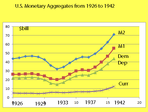
In 1928, due to what the US Federal Reserve believed was excessive speculation on Wall Street, its Board decided to contract the money supply by liquidating three-quarters of its holdings of US treasuries. By doing so, it reduced banking reserves.

How disruptive was this? According to Professor James Hamilton in his review of the Great Depression.

“In terms of the magnitudes consciously controlled by the Federal Reserve, it would have been difficult to design a more contractionary policy” (James Hamilton, “Monetary Factors in the Great Depression,” Journal of Monetary Economics, 1987).

We can see the downward impact on M2, M1 and other monetary aggregates over 1928/1929 in the following table (source: San Jose State University, Department of Economics).

Interest rate/debt stress

The Federal Reserve raised interest rates from 3.5 per cent to 5 per cent through 1928 and again to 6 per cent in August 1929.

Why the latter raise was required is somewhat of a puzzle. Economic growth had already softened in the first half of 1929 post the 1.5 per cent rate increase and contraction in money supply (source: Federal Reserve Bank of San Francisco, 1999).

Jobs decline

The impact of both the contraction in money supply and higher rates was felt amongst workers. Unemployment data for this period is somewhat inaccurate, but records from union membership databases show unemployment rising from 9 per cent in August 1929 to 11 per cent by October 1929 after the latter August rate rise.

The Result

As a whole, the reduction in money supply and higher interest rates put increasing pressure on jobs and consumption.

Less jobs begets less consumption/production which then culls more jobs and the cycle continues. If the decline in jobs/borrowing (and thus consumption) is significant enough, a recession is often the result.

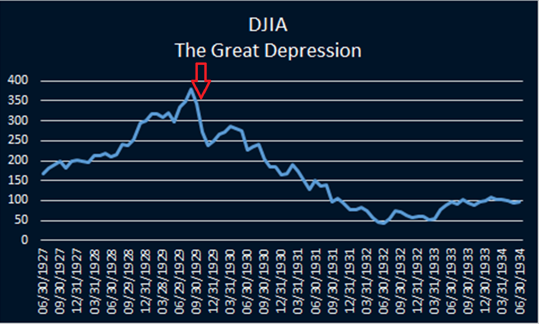
Naturally, less production for firms means lower near term earnings and more conservative future growth prospects. As such, stock prices tend to contract when recessions/depressions occur. The stock market capitulated from October 1929 into one of the greatest declines of all time.

Despite the onset of the depression in 1929, the money supply kept on contracting into the early 30’s due to restrictive monetary policies - exacerbating what may have been a more ordinary recession. Hawkish fiscal policy was also a major contributing factor.

To sum it up

The Great Depression is one example of how Vega Capital’s model can be applied to identify an economic calamity before it occurs. In the below table, I’ve noted 5 recessions (the 5 worst for stock markets over the past 50 years) along with the lead time our model provides (in months).

A positive lead time indicates that the model gave an early sign and negative means the model was late.

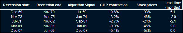
The results as shown are quite strong. Even with a signal which is 2 months late, the algorithm was able to capture the majority of the subsequent stock market decline (it notably takes many months for economists and the market to identify recessions in hindsight).

The model is currently advising caution through 2019/2020 and has not shown readings this negative since 2007, but we are yet to short the market outright.